Medical Visualization
A WebGL2 direct volume renderer for medical CT/MRI scans, with transfer functions and Lambertian lighting with soft shadows.
A browser-based direct volume renderer. It takes a preprocessed medical volume (CT, MRI, …), marches a ray through it for every pixel in a fragment shader, and lets you decide interactively what to look at: which tissue is visible, in which colour, and how it is lit.
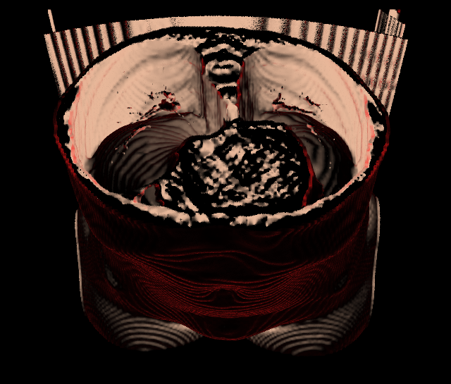
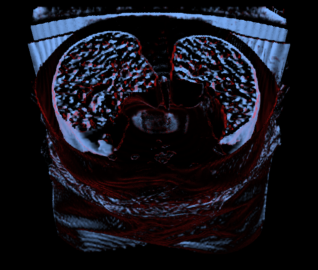
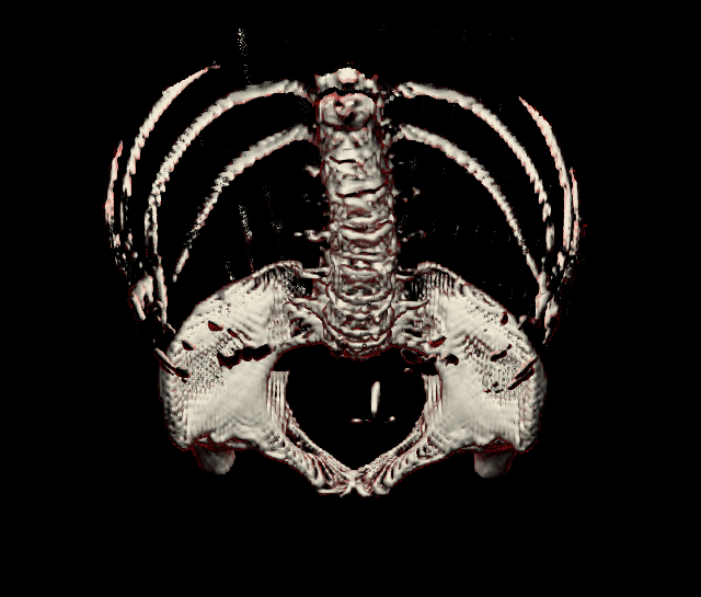
The same torso CT rendered in the browser with three transfer functions: the body surface, the lungs and the bone.
What the project is
This is a project of the Scientific Visualization course (MIRI-SV-MEDVIZ, UPC). The course provided a skeleton: a web page with an orbit camera, a transfer-function editor, light controls, and a first, partial (and partly incorrect) ray-marching shader. The work consisted of:
- Preparing volumetric data with SimpleITK and converting it to the raw text format the viewer reads (see Data preparation).
- Implementing the volume rendering in the fragment shader: ray-box intersection, compositing, and a transfer function chosen by the user.
- Implementing lighting: Lambert shading and shadows, hard and soft, with two ways of combining the shadow rays.
- Correcting the skeleton’s pipeline (sampling, opacity accumulation, normals, shadow rays) and adding an illustrative silhouette enhancement.
Everything that draws the image lives in one file, shaders/fragmentShader.glsl. The web page (camera, controls, loader) is the course’s base.
What was implemented
| Area | What the shader does |
|---|---|
| Ray setup | Every pixel casts a ray from the camera through the cube. A ray-box (slab) test gives the entry and exit points, and rays that miss the volume are discarded. |
| Sampling step | 0.5 x the smallest voxel size: two samples per voxel along the finest axis, which is the Nyquist-Shannon limit, so thin structures are not skipped. A small per-pixel random offset (jitter) hides the “wood grain” banding that regular sampling creates. |
| Compositing | Front-to-back with premultiplied alpha, and early ray termination once 95% opacity is reached. |
| Opacity | The opacity of a sample is corrected to the step length (1 - (1 - alpha)^(step / reference)), so the image does not change when the step size or the volume resolution does. Opaque surfaces are unaffected. |
| Transfer function | Trapezoid defined by four values in the volume’s own units (for a CT, Hounsfield units), plus one colour and a global opacity. |
| Normals | Normalised gradient of the original scalar field (central differences), not of the opacity. |
| Shading | Lambert (N . L). |
| Shadows | Rays from each sample towards the light, with their own entry/exit points, front-to-back opacity accumulation and early exit. Zero rays means no shadows, one ray gives a hard shadow, and several rays towards a disk-shaped area light give soft shadows. |
| Two shadow strategies | Percentage and Accumulation (explained in Lighting). |
| Silhouette | A Fresnel-like rim term (1 - abs(N . V))^p, gated so only real boundaries get an outline (see Silhouette enhancement). |
Running it
The page loads shaders over HTTP, so it has to be served (opening index.html directly will not work).
python3 -m http.server 8000Then open http://127.0.0.1:8000/ in a WebGL2-capable browser (Firefox or Chrome). The page loads gl-matrix and Chart.js from a CDN, so it needs an internet connection; nothing has to be installed with npm.
- Rotate: left click and drag on the image. Zoom: mouse wheel.
- Load Model: pick a
.rawfile and press Load Model. A new model can be loaded at any time. - Transfer function:
X0..X3(see below), the opacity slider and the colour picker. Reset returns to the default. - Light configuration:
ΛandΦ(direction), radius, distance, number of rays and strategy.
Data preparation
The website does not read clinical files directly. The notebook data_preparation.ipynb (SimpleITK) transforms a scan into the text .raw file the website loads: all the voxel values on one line, with the dimensions in the file name, <name>_<Z>_<Y>_<X>.raw.
Two volumes are used below: testingLight_15_30_30.raw, a small synthetic scene that came with the project and makes shadows easy to read, and out_100_128_128.raw, a torso CT prepared with the notebook.
Lighting
The light is set with the controls below. In the world the volume is a cube that goes from -1 to 1 on each axis.
| Parameter | What it does |
|---|---|
| Λ (lambda) and Φ (phi) | Direction of the light, as spherical coordinates around the centre of the cube. |
| Distance | How far the light is from the centre of the cube. |
| Radius | Size of the disk-shaped area light: the bigger it is, the softer the shadow edge. |
| Number of rays | 0: no shadows. 1: one ray to the centre of the light, a hard shadow. 2 or more: random rays to points on the disk, a soft shadow. |
| Strategy | How the rays of one point are combined: Percentage or Accumulation (below). |
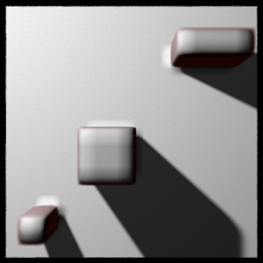
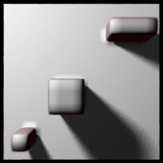
The images below use the test volume seen from the front, with Λ = 2.4, Φ = 0.8, distance = 3 and radius = 0.3.
Number of rays
One ray gives a hard shadow. With more rays every point sends its rays to different random points on the light, so the edge becomes a soft penumbra: grainy with few rays, and smoother the more rays there are, at a cost in speed. Shadows are dark grey, never black, because the shader keeps a minimum light visibility (0.2).
| 1 ray | 20 rays (Percentage) |
|---|---|
 |
 |
Percentage and Accumulation
Both strategies trace the same rays and differ in how they turn them into one visibility value between 0 (shadow) and 1 (lit):
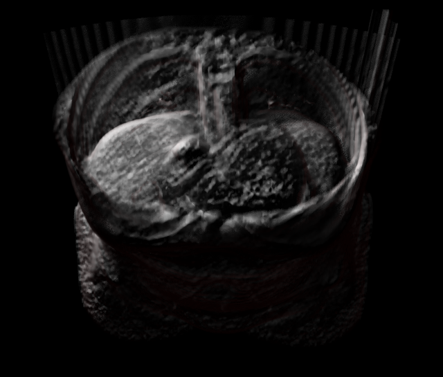
- Percentage: a ray is blocked only if it reaches full opacity on its way to the light. The visibility is the share of rays that are not blocked.
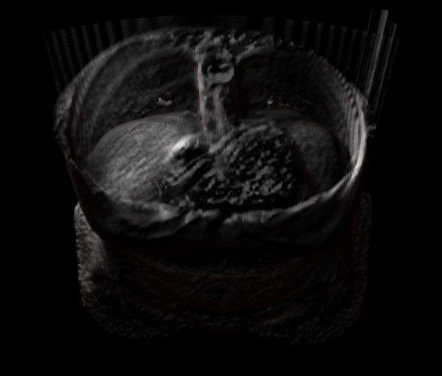
- Accumulation: every ray contributes the opacity it gathered. The visibility is
1 - the average opacity.
On opaque material, like the test volume above, each ray is either blocked or free, so both give practically the same picture. On translucent material most rays only gather part of the opacity: Percentage then treats nearly all of them as free (bright and flat), while Accumulation darkens the point in proportion to the material the light crosses. The example is a translucent render of the CT body (the body surface transfer function at a very low opacity), with 10 rays and radius 0.3:
| Percentage | Accumulation |
|---|---|
 |
 |
Transfer functions
The transfer function decides what is visible. It is a trapezoid over the values of the volume, defined by four numbers:
opacity
   ^      X1________X2
   |      /          \
   |     /            \
   |____/              \____
+---X0---------------X3------> voxel value- Below
X0and aboveX3: fully transparent. - From
X0toX1: opacity rises linearly. FromX1toX2: full opacity. FromX2toX3: it falls again. - The opacity slider scales the whole curve and the colour picker sets the colour of everything that is visible.
The values are the volume’s own units, so for a CT they are Hounsfield units, and the same anatomy always sits in the same place. For the torso CT used here:
| Tissue | Approximate HU |
|---|---|
| Air | below -950 |
| Lung | -950 to -700 |
| Fat and soft tissue | -150 to 150 |
| Bone | above 250 |
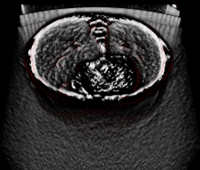
Choosing the trapezoid to match one of those ranges is how the same scan can show different things. All the images below use the same camera (below the volume and looking up along the slice axis), no shadows, and only the transfer function changes.
 A. Default ramp |
B. Body surface |
C. Lungs |
D. Bone |
| X0 | X1 | X2 | X3 | Colour | |
|---|---|---|---|---|---|
| A. Default ramp | -1024 | 1637 | 1637 | 1637 | white |
| B. Body surface | -300 | -100 | 1637 | 1637 | skin #e8b89a |
| C. Lungs | -950 | -880 | -750 | -600 | blue #7fb4ff |
| D. Bone | 250 | 350 | 1637 | 1637 | ivory #f2ecd8 |
The opacity slider is at 1 in all of them.
- A, the starting point. This is what the page shows when a model is loaded: opacity grows from the lowest to the highest value across the whole range. Almost everything is a little visible at once, so the result is a noisy grey block, and the CT table (the stripes at the top) is as prominent as the patient. It shows the volume, but not the anatomy.
- B, the body surface. Everything from fat upwards (above about -100 HU) is opaque, in a skin tone, while air and lung stay transparent. The result is the body wall seen from below, with the table, and the cut face of the volume shows what is inside.
- C, the lungs. A window around the lung values makes the lungs the main thing you see, in blue (with a faint trace of the body surface, where skin and air blend). The texture of the lung tissue comes out speckled, which is real noise in the scan that a narrow window makes visible.
- D, the bone. A window that starts at 250 HU keeps only bone: the ribs, the spine and the pelvis appear clean and detached from the rest of the body. It is the clearest result of the set.
Silhouette enhancement
To make the shape of structures easier to read, the renderer can outline the places where the surface is seen edge-on. At every sample the shader computes a weight
w = (1 - |N . V|)^pwhere N is the surface normal (the same one used for Lambert shading), V is the direction to the viewer, and p > 1 sets how sharp the outline is. w is close to 0 where the surface faces the camera and close to 1 where it is seen at a grazing angle. The strongest response along the ray tints the final colour towards the outline colour, in proportion to how opaque the ray became.
To keep it stable across datasets and transfer functions, the outline is gated by how much the opacity changes over two voxels. That is about 0 in noise and in flat regions, and about 1 at a real boundary of what is being rendered. So outlines appear at boundaries, not on the grain of a noisy scan, and the gate does not depend on the range of values of the volume. The sharpness p (SIL_P, 4), the strength (SIL_STRENGTH, 0.6) and the colour (SIL_COLOR, red) are constants at the top of the shader. The red edges on the CT images above are this effect.